本文翻译自 Jonas Kristoffer Lindeløv 的 Common statistical tests are linear models (or: how to teach stats),翻译工作已获得原作授权。本翻译工作首发于统计之都网站和微信公众号上。
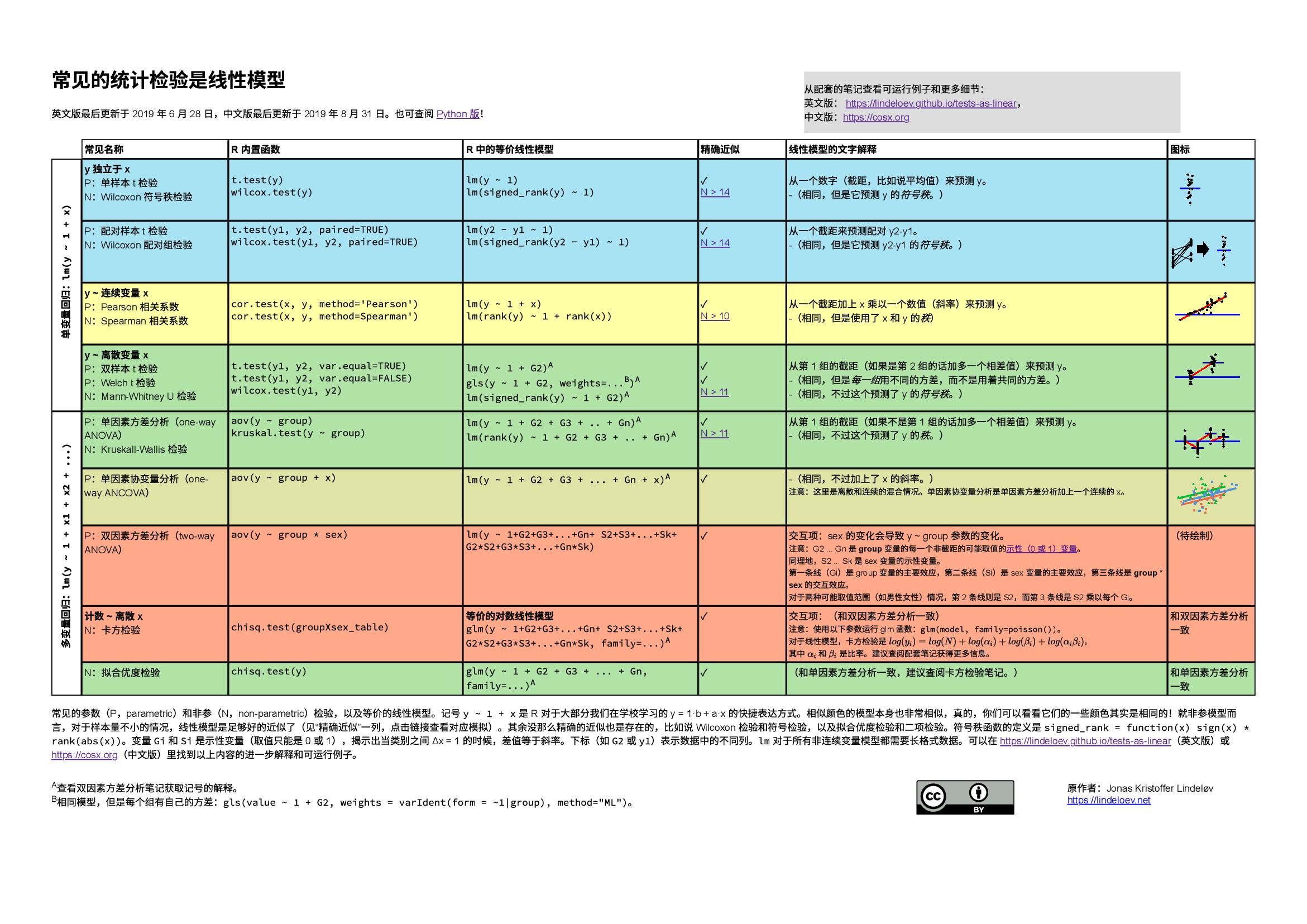
本文将常见的参数和“非参”数检验统一用线性模型来表示,在同一个框架下, 我们可以看到不同检验之间的许多相似之处,极富思考性和启发性。点击链接可获得一份 PDF 电子版 或 HTML 网页版。
1 常见检验的本质
大部分常见的统计模型(t 检验、相关性检验、方差分析(ANOVA)、卡方检验等) 是线性模型的特殊情况或者是非常好的近似。这种优雅的简洁性意味着我们学习起来不需要掌握太多的技巧。具体来说,这都来源于大部分学生从高中就学习的模型:\(y = a \cdot x + b\)。 然而很不幸的是,统计入门课程通常把各种检验分开教学,给学生和老师们增加了很多不必要的麻烦。在学习每一个检验的基本假设时,如果不是从线性模型切入,而是每个检验都死记硬背,这种复杂性又会成倍增加。因此,我认为先教线性模型,然后对线性模型的一些特殊形式进行改名是一种优秀的教学策略,这有助于更深刻地理解假设检验。线性模型在频率学派、贝叶斯学派和基于置换的U检验的统计推断之间是相通的,对初学者而言,从模型开始比从 P 值、第 I 类错误、贝叶斯因子或其它地方更为友好。
在入门课程教授“非参”数检验的时候,可以避开 骗小孩 的手段,直接告诉学生“非参”检验其实就是和秩相关的参数检验。对学生来说,接受秩的概念比相信你可以神奇地放弃各种假设好的多。实际上,在统计软件 JASP 里,“非参”检验的贝叶斯等价模型就是使用 潜秩(Latent Rank)来实现的。频率学派的“非参”检验在样本量 \(N > 15\) 的时非常准确。

在来源和教材两章节,有很多类似(尽管更为散乱)的材料。我希望你们可以一起来提供优化建议,或者直接在 Github 提交修改。让我们一起来使本文章变得更棒!
2 设置和示例数据
如果你想查看函数和本笔记的其它设置的话,可以展开这片代码查看:
# 加载必要的 R 包用于处理数据和绘图
library(tidyverse)
library(patchwork)
library(broom)

# 设置随机数种子复现本文结果
set.seed(40)

# 生成已知参数的服从正态分布的随机数
rnorm_fixed <- function(N, mu = 0, sd = 1)
  scale(rnorm(N)) * sd + mu

# 图形风格
theme_axis <- function(P, jitter = FALSE,
                       xlim = c(-0.5, 2),
                       ylim = c(-0.5, 2),
                       legend.position = NULL) {
  P <- P + theme_bw(15) +
    geom_segment(
      x = -1000, xend = 1000,
      y = 0, yend = 0,
      lty = 2, color = "dark gray", lwd = 0.5
    ) +
    geom_segment(
      x = 0, xend = 0,
      y = -1000, yend = 1000,
      lty = 2, color = "dark gray", lwd = 0.5
    ) +
    coord_cartesian(xlim = xlim, ylim = ylim) +
    theme(
      axis.title = element_blank(),
      axis.text = element_blank(),
      axis.ticks = element_blank(),
      panel.border = element_blank(),
      panel.grid = element_blank(),
      legend.position = legend.position
    )

  # 是否设置抖动
  if (jitter) {
    P + geom_jitter(width = 0.1, size = 2)
  }
  else {
    P + geom_point(size = 2)
  }
}一开始,我们简单点,使用三组正态分布数据,且整理为宽(a、b、c)和长(value、group)格式:
# Wide format (sort of)
# y = rnorm_fixed(50, mu=0.3, sd=2)  # Almost zero mean.
y <- c(rnorm(15), exp(rnorm(15)), runif(20, min = -3, max = 0)) # Almost zero mean, not normal
x <- rnorm_fixed(50, mu = 0, sd = 1) # Used in correlation where this is on x-axis
y2 <- rnorm_fixed(50, mu = 0.5, sd = 1.5) # Used in two means

# Long format data with indicator
value <- c(y, y2)
group <- rep(c("y1", "y2"), each = 50)
3 Pearson 相关性和 Spearman 相关性
3.1 理论:作为线性模型
模型:\(y\) 的形式是一个斜率(\(\beta_1\))乘以 \(x\) 加上一个截距(\(\beta_0\)),也就是一条直线。
\[y = \beta_0 + \beta_1 x \qquad \mathcal{H}_0: \beta_1 = 0\]
以上模型,实际上是我们熟悉的旧公式 \(y = ax + b\) (这里书写顺序变为 \(y = b + ax\))1的一个更数学化的表达。在 R 软件里面,我们比较懒,所以写成了 y ~ 1 + x,R 对此理解为 \(y = 1\times\mathrm{数} + x\times\mathrm{另一个数}\),而且,t 检验,线性回归等等都只是去寻找能够最好地预测 \(y\) 的数字。
无论你怎么书写,截距(\(\beta_0\))和斜率(\(\beta_1\))都可以确定一条直线:
# Fixed correlation
D_correlation <- data.frame(MASS::mvrnorm(30,
  mu = c(0.9, 0.9),
  Sigma = matrix(c(1, 0.8, 1, 0.8), ncol = 2),
  empirical = TRUE
)) # Correlated data

# Add labels (for next plot)
D_correlation$label_num <- sprintf("(%.1f,%.1f)", D_correlation$X1, D_correlation$X2)
D_correlation$label_rank <- sprintf("(%i,%i)", rank(D_correlation$X1), rank(D_correlation$X2))

# Plot it
fit <- lm(I(X2 * 0.5 + 0.4) ~ I(X1 * 0.5 + 0.2), D_correlation)
intercept_pearson <- coefficients(fit)[1]

P_pearson <- ggplot(D_correlation, aes(x = X1 * 0.5 + 0.2, y = X2 * 0.5 + 0.4)) +
  geom_smooth(method = lm, se = FALSE, lwd = 2, aes(colour = "beta_1")) +
  geom_segment(
    x = -100, xend = 100,
    y = intercept_pearson, yend = intercept_pearson,
    lwd = 2, aes(color = "beta_0")
  ) +
  scale_color_manual(name = NULL, values = c("blue", "red"),
                     labels = c(bquote(beta[0] * " (intercept)"),
                                bquote(beta[1] * " (slope)")))

theme_axis(P_pearson, legend.position = c(0.4, 0.9))
这是所谓的回归模型,当右边有多个 \(\beta\) 和自变量相乘的时候,它扩展为多元回归。以下的所有模型,从 单样本 t 检验到 双因素方差分析,都是这个模型的特殊形式,不多不少。
顾名思义,Spearman 秩相关系数就是 \(x\) 和 \(y\) 的秩变换后的Pearson 相关系数:
\[\mathrm{rank}(y) = \beta_0 + \beta_1 \cdot \mathrm{rank}(x) \qquad \mathcal{H}_0: \beta_1 = 0\]
很快我就会介绍 秩 这个概念。现在,线性模型的相关系数等价于“真正的” Pearson 相关系数,但 P 值是近似值,这个近似值适用于 \(N>10\) 的情况,并且在 \(N > 20\) 时 几乎完美。
很多学生都没有意识到这么漂亮和神奇的等价关系!给线性回归带上数据标签来,我们可立刻看到秩转换过程:
# Spearman intercept
intercept_spearman <- coefficients(lm(rank(X2) ~ rank(X1), D_correlation))[1]

# Spearman plot
P_spearman <- ggplot(D_correlation, aes(x = rank(X1), y = rank(X2))) +
  geom_smooth(method = lm, se = FALSE, lwd = 2, aes(color = "beta_1")) +
  geom_text(aes(label = label_rank), nudge_y = 1, size = 3, color = "dark gray") +
  geom_segment(
    x = -100, xend = 100,
    y = intercept_spearman, yend = intercept_spearman,
    lwd = 2, aes(color = "beta_0")
  ) +
  scale_color_manual(name = NULL, values = c("blue", "red"),
                     labels = c(bquote(beta[0] * " (intercept)"),
                                bquote(beta[1] * " (slope)")))

# 用 patchwork 包把图组合在一块
(theme_axis(P_pearson, legend.position = c(0.5, 0.1)) +
    geom_text(aes(label = label_num), nudge_y = 0.1, size = 3, color = "dark gray") +
    labs(title = "         Pearson")) +
(theme_axis(P_spearman, xlim = c(-7.5, 30), ylim = c(-7.5, 30),
              legend.position = c(0.5, 0.1)) +
     labs(title = "         Spearman"))
3.2 理论:秩转换
对于一串数字,秩(rank)意思是使用它们的排序号来替换它们(第 1 最小的,第 2 最小的,第 3 最小的,以此类推)。因此 rank(c(3.6, 3.4, -5.0, 8.2)) 的秩转换结果是 3, 2, 1, 4。从上面的图形里看出来了吗?符号秩是一样的,先根据绝对值排序,再添加上数值前面的符号。所以上面的符号秩是 2, 1, -3, 4。用代码表示如下:
signed_rank = function(x) sign(x) * rank(abs(x))我希望我说秩很容易理解的时候没有冒犯到其他人。这就是转换大部分“非参”数检验到它们的对应参数检验所要做的全部事情!一个重要的推论是很多“非参”检验和它们的对应参数检验版本都有一致的参数:均值、标准差、齐次方差等等 —— 区别在于它们是在秩转换后的数据上计算的。这是为什么我把“非参”用引号包起来。
3.2.1 R 代码:Pearson 相关系数
在 R 里运行这些模型再容易不过了。它们产生相同的 p 值和 t 值,但是这里有个问题:lm 返回斜率,尽管它通常比相关系数 r 更容易理解和反映了更多信息,但你依然想得到 r 值。幸运地,如果 x 和 y 有相同的标准差,斜率就会变成 r。所以,在这里我们使用 scale(x) 使得 \(SD(x) = 1.0\) 和 \(SD(y) = 1.0\):
a <- cor.test(y, x, method = "pearson") # Built-in
b <- lm(y ~ 1 + x) # Equivalent linear model: y = Beta0*1 + Beta1*x
c <- lm(scale(y) ~ 1 + scale(x)) # On scaled vars to recover r
结果:
##
##  Pearson's product-moment correlation
##
## data:  y and x
## t = -0.33651, df = 48, p-value = 0.738
## alternative hypothesis: true correlation is not equal to 0
## 95 percent confidence interval:
##  -0.3225066  0.2329799
## sample estimates:
##         cor
## -0.04851394
##
##
## Call:
## lm(formula = y ~ 1 + x)
##
## Residuals:
##     Min      1Q  Median      3Q     Max
## -2.6265 -1.1753 -0.3718  0.6607  5.7109
##
## Coefficients:
##             Estimate Std. Error t value Pr(>|t|)
## (Intercept) -0.09522    0.25647  -0.371    0.712
## x           -0.08718    0.25907  -0.337    0.738
##
## Residual standard error: 1.814 on 48 degrees of freedom
## Multiple R-squared:  0.002354,   Adjusted R-squared:  -0.01843
## F-statistic: 0.1132 on 1 and 48 DF,  p-value: 0.738
##
##
## Call:
## lm(formula = scale(y) ~ 1 + scale(x))
##
## Residuals:
##     Min      1Q  Median      3Q     Max
## -1.4616 -0.6541 -0.2069  0.3677  3.1780
##
## Coefficients:
##               Estimate Std. Error t value Pr(>|t|)
## (Intercept)  1.722e-17  1.427e-01   0.000    1.000
## scale(x)    -4.851e-02  1.442e-01  -0.337    0.738
##
## Residual standard error: 1.009 on 48 degrees of freedom
## Multiple R-squared:  0.002354,   Adjusted R-squared:  -0.01843
## F-statistic: 0.1132 on 1 and 48 DF,  p-value: 0.738
置信区间没有完全一致,但是非常相近。
3.2.2 R 代码:Spearman 相关系数
注意,我们可以把斜率解释为:对于每一 \(x\) 的秩的变化,所获得的相应 \(y\) 的秩的变化。我认为这个数字非常有趣。然而,截距更难解释,因为它定义在 \(\mathrm{rank}(x) = 0\) 的时候,然而这其实是不可能的,因为 x 是从 1 开始的。
查看相同的 r (即这里的 rho) 和 p:
# Spearman correlation
a <- cor.test(y, x, method = "spearman") # Built-in
b <- lm(rank(y) ~ 1 + rank(x)) # Equivalent linear model
让我们看一下结果:
##
##  Spearman's rank correlation rho
##
## data:  y and x
## S = 21956, p-value = 0.7072
## alternative hypothesis: true rho is not equal to 0
## sample estimates:
##         rho
## -0.05430972
##
##
## Call:
## lm(formula = rank(y) ~ 1 + rank(x))
##
## Residuals:
##      Min       1Q   Median       3Q      Max
## -23.8211 -12.0056  -0.0272  12.5215  25.6677
##
## Coefficients:
##             Estimate Std. Error t value Pr(>|t|)
## (Intercept) 26.88490    4.22287   6.366 6.89e-08 ***
## rank(x)     -0.05431    0.14412  -0.377    0.708
## ---
## Signif. codes:  0 '***' 0.001 '**' 0.01 '*' 0.05 '.' 0.1 ' ' 1
##
## Residual standard error: 14.71 on 48 degrees of freedom
## Multiple R-squared:  0.00295,    Adjusted R-squared:  -0.01782
## F-statistic: 0.142 on 1 and 48 DF,  p-value: 0.708
4 单均值
4.1 单样本 t 检验和 Wilcoxon 符号秩检验
4.1.1 理论:作为线性模型
t 检验模型:单独一个数字来预测 \(y\)。
\[y = \beta_0 \qquad \mathcal{H}_0: \beta_0 = 0\]
换句话说,这是我们所熟悉的 \(y = \beta_0 + \beta_1*x\),只是最后一项消失了,因为 \(x\) 不存在了(等价于 \(x=0\),见下方左图)。以上模型,一旦用 \(y\) 的 符号秩来替换了 \(y\) 本身(见下方右图),就和Wilcoxon 符号秩检验非常相近。
\[\mathrm{signed\_rank}(y) = \beta_0\]
这个近似对于样本量大于 14 的情况已足够好,对于大于 50 的情况 接近完美。
# T-test
D_t1 <- data.frame(
  y = rnorm_fixed(20, 0.5, 0.6),
  x = runif(20, 0.93, 1.07)
) # Fix mean and SD

P_t1 <- ggplot(D_t1, aes(y = y, x = 0)) +
  stat_summary(
    fun.y = mean, geom = "errorbar",
    aes(ymax = ..y.., ymin = ..y.., color = "beta_0"), lwd = 2
  ) +
  scale_color_manual(
    name = NULL, values = c("blue"),
    labels = c(bquote(beta[0] * " (intercept)"))
  ) +
  geom_text(aes(label = round(y, 1)), nudge_x = 0.2, size = 3, color = "dark gray") +
  labs(title = "         T-test")

# Wilcoxon
D_t1_rank <- data.frame(y = signed_rank(D_t1$y))

P_t1_rank <- ggplot(D_t1_rank, aes(y = y, x = 0)) +
  stat_summary(
    fun.y = mean, geom = "errorbar",
    aes(ymax = ..y.., ymin = ..y.., color = "beta_0"), lwd = 2
  ) +
  scale_color_manual(
    name = NULL, values = c("blue"),
    labels = c(bquote(beta[0] * " (intercept)"))
  ) +
  geom_text(aes(label = y), nudge_x = 0.2, size = 3, color = "dark gray") +
  labs(title = "         Wilcoxon")

# Stich together using patchwork
theme_axis(P_t1, ylim = c(-1, 2), legend.position = c(0.6, 0.1)) +
theme_axis(P_t1_rank, ylim = NULL, legend.position = c(0.6, 0.1))
4.1.2 R 代码:单样本 t 检验
尝试运行以下 R 代码,确认线性模型(lm)和内置的 t.test 产生相同的 \(t\)、\(p\)、\(r\)。lm 的输出没有置信区间,但是你可以用 confint(lm(...)) 来确认结果也是相同的:
# Built-in t-test
a <- t.test(y)

# Equivalent linear model: intercept-only
b <- lm(y ~ 1)
结果:
##
##  One Sample t-test
##
## data:  y
## t = -0.37466, df = 49, p-value = 0.7095
## alternative hypothesis: true mean is not equal to 0
## 95 percent confidence interval:
##  -0.6059252  0.4154934
## sample estimates:
##   mean of x
## -0.09521589
##
##
## Call:
## lm(formula = y ~ 1)
##
## Residuals:
##     Min      1Q  Median      3Q     Max
## -2.6877 -1.1888 -0.3123  0.5868  5.5883
##
## Coefficients:
##             Estimate Std. Error t value Pr(>|t|)
## (Intercept) -0.09522    0.25414  -0.375     0.71
##
## Residual standard error: 1.797 on 49 degrees of freedom
4.1.3 R 代码:Wilcoxon 符号秩检验
除了一致的 p 值,lm 也提供了符号秩均值,我发现这个数字非常有信息量。
# Built-in
a <- wilcox.test(y)

# Equivalent linear model
b <- lm(signed_rank(y) ~ 1) # See? Same model as above, just on signed ranks

# Bonus: of course also works for one-sample t-test
c <- t.test(signed_rank(y))
结果:
##
##  Wilcoxon signed rank test with continuity correction
##
## data:  y
## V = 508, p-value = 0.213
## alternative hypothesis: true location is not equal to 0
##
##
## Call:
## lm(formula = signed_rank(y) ~ 1)
##
## Residuals:
##    Min     1Q Median     3Q    Max
## -41.82 -22.57  -5.32  18.68  55.18
##
## Coefficients:
##             Estimate Std. Error t value Pr(>|t|)
## (Intercept)    -5.18       4.12  -1.257    0.215
##
## Residual standard error: 29.13 on 49 degrees of freedom
##
##
##  One Sample t-test
##
## data:  signed_rank(y)
## t = -1.2573, df = 49, p-value = 0.2146
## alternative hypothesis: true mean is not equal to 0
## 95 percent confidence interval:
##  -13.459062   3.099062
## sample estimates:
## mean of x
##     -5.18
4.2 配对样本 t 检验和 Wilcoxon 配对组检验
4.2.1 理论:作为线性模型
t 检验模型:一个数字(截距)来预测组间之差。
\[y_2 - y_1 = \beta_0 \qquad \mathcal{H}_0: \beta_0 = 0\]
这意味着只有一个 \(y = y_2 - y_1\) 需要预测,而且它变成了对于组间之差的 单样本 t 检验。因此可视化效果和单样本 t 检验是相同的。冒着过度复杂化简单作差的风险,你可以认为这些组间之差是斜率(见图的左半部分),我们也可以用 \(y\) 的差来表达(见图的右半部分):
# Data for plot
N <- nrow(D_t1)
start <- rnorm_fixed(N, 0.2, 0.3)
D_tpaired <- data.frame(
  x = rep(c(0, 1), each = N),
  y = c(start, start + D_t1$y),
  id = 1:N
)

# Plot
P_tpaired <- ggplot(D_tpaired, aes(x = x, y = y)) +
  geom_line(aes(group = id)) +
  labs(title = "          Pairs")

# Use patchwork to put them side-by-side
theme_axis(P_tpaired) +
theme_axis(P_t1, legend.position = c(0.6, 0.1))
类似地,Wilcoxon 配对组和Wilcoxon 符号秩的唯一差别,就是它对配对的差 \(y-x\) 的符号秩进行检验。
\(\mathrm{signed\_rank}(y_2-y_1) = \beta_0 \qquad \mathcal{H}_0: \beta_0 = 0\)
4.2.2 R 代码:配对样本 t 检验
a <- t.test(y, y2, paired = TRUE) # Built-in paired t-test
b <- lm(y - y2 ~ 1) # Equivalent linear model
结果:
##
##  Paired t-test
##
## data:  y and y2
## t = -1.7108, df = 49, p-value = 0.09345
## alternative hypothesis: true difference in means is not equal to 0
## 95 percent confidence interval:
##  -1.2943926  0.1039608
## sample estimates:
## mean of the differences
##              -0.5952159
##
##
## Call:
## lm(formula = y - y2 ~ 1)
##
## Residuals:
##     Min      1Q  Median      3Q     Max
## -5.9699 -1.4071 -0.0062  1.0771  7.2116
##
## Coefficients:
##             Estimate Std. Error t value Pr(>|t|)
## (Intercept)  -0.5952     0.3479  -1.711   0.0934 .
## ---
## Signif. codes:  0 '***' 0.001 '**' 0.01 '*' 0.05 '.' 0.1 ' ' 1
##
## Residual standard error: 2.46 on 49 degrees of freedom
4.2.3 R 代码:Wilcoxon 配对组检验
我们再一次运用符号秩转换技巧。这依然是近似值,但是非常接近:
# Built-in Wilcoxon matched pairs
a <- wilcox.test(y, y2, paired = TRUE)

# Equivalent linear model:
b <- lm(signed_rank(y - y2) ~ 1)

# Bonus: identical to one-sample t-test ong signed ranks
c <- t.test(signed_rank(y - y2))
结果:
##
##  Wilcoxon signed rank test with continuity correction
##
## data:  y and y2
## V = 429, p-value = 0.04466
## alternative hypothesis: true location shift is not equal to 0
##
##
## Call:
## lm(formula = signed_rank(y - y2) ~ 1)
##
## Residuals:
##    Min     1Q Median     3Q    Max
## -40.66 -23.16  -4.66  20.84  58.34
##
## Coefficients:
##             Estimate Std. Error t value Pr(>|t|)
## (Intercept)   -8.340      4.013  -2.078   0.0429 *
## ---
## Signif. codes:  0 '***' 0.001 '**' 0.01 '*' 0.05 '.' 0.1 ' ' 1
##
## Residual standard error: 28.37 on 49 degrees of freedom
##
##
##  One Sample t-test
##
## data:  signed_rank(y - y2)
## t = -2.0785, df = 49, p-value = 0.04293
## alternative hypothesis: true mean is not equal to 0
## 95 percent confidence interval:
##  -16.4036084  -0.2763916
## sample estimates:
## mean of x
## -8.34对于大样本量(\(N >> 100\)),这计算方式某种程度上比较接近符号检验。但是本例子中这种近似效果较差。
5 双均值
5.1 独立 t 检验和 Mann-Whitney U 检验
5.1.1 理论:作为线性模型
独立 t 检验模型:两个均值来预测 \(y\)。
\[y_i = \beta_0 + \beta_1 x_i \qquad \mathcal{H}_0: \beta_1 = 0\]
上式中,\(x_i\) 是示性变量(0 或 1),用于示意数据点 \(i\) 是从一个组里采样还是另一个组里采样的。 示性变量 indicator variable 或哑变量 dummy variable 或者 one-hot 编码 存在于很多线性模型当中,我们很快就会看到它有什么用途。
Mann-Whitney U 检验(也被称为两个独立组的 Wilcoxon 秩和检验;这次没有符号秩了)是有着非常接近的近似的相同模型,除了它不是在原有值而是在 \(x\) 和 \(y\) 的秩上计算的:
\[\mathrm{rank}(y_i) = \beta_0 + \beta_1 x_i \qquad \mathcal{H}_0: \beta_1 = 0\]
对我来说,这种等价性使“非参”统计量更容易理解了。这种近似在每个组样本量大于 11 的时候比较合适,在每个组样本量大于 30 的时候看起来 相当完美.
5.1.2 理论:示性变量
示性变量可以用图像来帮助理解。这个变量在 x 轴,所以第一个组的数据点位于 \(x = 0\),第二个组的位于 \(x = 1\)。然后 \(\beta_0\) 是截距(蓝线),\(\beta_1\) 是两个均值之间的斜率(红线)。为什么?因为当 \(\Delta x = 1\) 的时候,斜率等于相差值:
\[\mathrm{slope} = \Delta y / \Delta x = \Delta y / 1 = \Delta y = \mathrm{difference}\]
奇迹啊!即使类别之间的差值也可以用线性模型来表达,这真的是一把瑞士军刀!
# Data
N <- 20 # Number of data points per group
D_t2 <- data.frame(
  x = rep(c(0, 1), each = N),
  y = c(rnorm_fixed(N, 0.3, 0.3), rnorm_fixed(N, 1.3, 0.3))
)

# Plot
P_t2 <- ggplot(D_t2, aes(x = x, y = y)) +
  stat_summary(
    fun.y = mean, geom = "errorbar",
    aes(ymax = ..y.., ymin = ..y.., color = "something"), lwd = 2
  ) +
  geom_segment(x = -10, xend = 10, y = 0.3, yend = 0.3, lwd = 2, aes(color = "beta_0")) +
  geom_segment(x = 0, xend = 1, y = 0.3, yend = 1.3, lwd = 2, aes(color = "beta_1")) +
  scale_color_manual(
    name = NULL, values = c("blue", "red", "darkblue"),
    labels = c(
      bquote(beta[0] * " (group 1 mean)"),
      bquote(beta[1] * " (slope = difference)"),
      bquote(beta[0] + beta[1] %.% 1 * " (group 2 mean)")
    )
  )
# scale_x_discrete(breaks=c(0.5, 1.5), labels=c('1', '2'))

theme_axis(P_t2, jitter = TRUE, xlim = c(-0.3, 2), legend.position = c(0.53, 0.08))
5.1.3 理论:示性变量(后续)
如果你觉得你理解了示性变量了,可以直接跳到下一章节。这里是对示性变量更为详细的解释:
如果数据点采样自第一个组,即 \(x_i = 0\),模型就会变成 \(y = \beta_0 + \beta_1 \cdot 0 = \beta_0\)。换句话说,模型预测的值是 \(beta_0\)。这些数据点的均值 \(\beta\) 是最好的预测,而 \(\beta_0\) 是第 1 组的均值。
另一方面,采样自第二个组的数据点有 \(x_i = 1\),所以模型变成了 \(y_i = \beta_0 + \beta_1\cdot 1 = \beta_0 + \beta_1\)。换句话说,我们加上了 \(\beta_1\),从第一组的均值移动到了第二组的均值。所以 \(\beta_1\) 成为了两个组的均值之差。
举个例子,假设第 1 组人是 25 岁(\(\beta_0 = 25\)),第 2 组人 28 岁(\(\beta_1 = 3\)),那么对于第 1 组的人的模型是 \(y = 25 + 3 \cdot 0 = 25\),第 2 组的人的模型是 \(y = 25 + 3 \cdot 1 = 28\)。
呼,搞定!对于初学者,理解示性变量需要一些时间,但是只需要懂得加法和乘法就能上手了!
5.1.4 R 代码:独立 t 检验
提醒一下,当我们在 R 里写 y ~ 1 + x,它是 \(y = \beta_0 \cdot 1 + \beta_1 \cdot x\) 的简写,R 会为你计算 \(\beta\) 值。因此,y ~ 1 + x 是 R 里面表达 \(y = a \cdot x + b\) 的形式。
注意相等的 t、df、p和估计值。我们可以用 confint(lm(...)) 获得置信区间。
# Built-in independent t-test on wide data
a <- t.test(y, y2, var.equal = TRUE)

# Be explicit about the underlying linear model by hand-dummy-coding:
group_y2 <- ifelse(group == "y2", 1, 0) # 1 if group == y2, 0 otherwise
b <- lm(value ~ 1 + group_y2) # Using our hand-made dummy regressor

# Note: We could also do the dummy-coding in the model
# specification itself. Same result.
c <- lm(value ~ 1 + I(group == "y2"))
结果:
##
##  Two Sample t-test
##
## data:  y and y2
## t = -1.798, df = 98, p-value = 0.07525
## alternative hypothesis: true difference in means is not equal to 0
## 95 percent confidence interval:
##  -1.25214980  0.06171803
## sample estimates:
##   mean of x   mean of y
## -0.09521589  0.50000000
##
##
## Call:
## lm(formula = value ~ 1 + group_y2)
##
## Residuals:
##     Min      1Q  Median      3Q     Max
## -2.6877 -1.0311 -0.2435  0.6106  5.5883
##
## Coefficients:
##             Estimate Std. Error t value Pr(>|t|)
## (Intercept) -0.09522    0.23408  -0.407   0.6851
## group_y2     0.59522    0.33104   1.798   0.0753 .
## ---
## Signif. codes:  0 '***' 0.001 '**' 0.01 '*' 0.05 '.' 0.1 ' ' 1
##
## Residual standard error: 1.655 on 98 degrees of freedom
## Multiple R-squared:  0.03194,    Adjusted R-squared:  0.02206
## F-statistic: 3.233 on 1 and 98 DF,  p-value: 0.07525
##
##
## Call:
## lm(formula = value ~ 1 + I(group == "y2"))
##
## Residuals:
##     Min      1Q  Median      3Q     Max
## -2.6877 -1.0311 -0.2435  0.6106  5.5883
##
## Coefficients:
##                      Estimate Std. Error t value Pr(>|t|)
## (Intercept)          -0.09522    0.23408  -0.407   0.6851
## I(group == "y2")TRUE  0.59522    0.33104   1.798   0.0753 .
## ---
## Signif. codes:  0 '***' 0.001 '**' 0.01 '*' 0.05 '.' 0.1 ' ' 1
##
## Residual standard error: 1.655 on 98 degrees of freedom
## Multiple R-squared:  0.03194,    Adjusted R-squared:  0.02206
## F-statistic: 3.233 on 1 and 98 DF,  p-value: 0.07525
5.1.5 R 代码:Mann-Whitney U 检验
# Wilcoxon / Mann-Whitney U
a <- wilcox.test(y, y2)

# As linear model with our dummy-coded group_y2:
b <- lm(rank(value) ~ 1 + group_y2) # compare to linear model above
##
## Wilcoxon rank sum test with continuity correction
##
## data: y and y2
## W = 924, p-value = 0.02484
## alternative hypothesis: true location shift is not equal to 0
##
##
## Call:
## lm(formula = rank(value) ~ 1 + group_y2)
##
## Residuals:
## Min 1Q Median 3Q Max
## -49.02 -22.26 -1.50 23.27 56.02
##
## Coefficients:
## Estimate Std. Error t value Pr(>|t|)
## (Intercept) 43.980 4.017 10.948 <2e-16 ***
## group_y2 13.040 5.681 2.295 0.0238 *
## ---
## Signif. codes: 0 '***' 0.001 '**' 0.01 '*' 0.05 '.' 0.1 ' ' 1
##
## Residual standard error: 28.41 on 98 degrees of freedom
## Multiple R-squared: 0.05102, Adjusted R-squared: 0.04133
## F-statistic: 5.269 on 1 and 98 DF, p-value: 0.023855.2 Welch t 检验
这等价于以上(学生)独立 t 检验,除了学生 t 检验假设同方差,而 Welch t 检验 没有这个假设。所以线性模型是相同的,区别在于,我们对每一个组指定一个方差。我们可用 nlme 包(查阅细节):
# Built-in
a <- t.test(y, y2, var.equal = FALSE)

# As linear model with per-group variances
b <- nlme::gls(value ~ 1 + group_y2, method = "ML",
               weights = nlme::varIdent(form = ~ 1 | group))
结果:
##
##  Welch Two Sample t-test
##
## data:  y and y2
## t = -1.798, df = 94.966, p-value = 0.07535
## alternative hypothesis: true difference in means is not equal to 0
## 95 percent confidence interval:
##  -1.25241218  0.06198041
## sample estimates:
##   mean of x   mean of y
## -0.09521589  0.50000000
##
## Generalized least squares fit by maximum likelihood
##   Model: value ~ 1 + group_y2
##   Data: NULL
##        AIC     BIC    logLik
##   388.9273 399.348 -190.4636
##
## Variance function:
##  Structure: Different standard deviations per stratum
##  Formula: ~1 | group
##  Parameter estimates:
##        y1        y2
## 1.0000000 0.8347122
##
## Coefficients:
##                  Value Std.Error    t-value p-value
## (Intercept) -0.0952159 0.2541379 -0.3746623  0.7087
## group_y2     0.5952159 0.3310379  1.7980295  0.0753
##
##  Correlation:
##          (Intr)
## group_y2 -0.768
##
## Standardized residuals:
##        Min         Q1        Med         Q3        Max
## -1.5789902 -0.6351823 -0.1639999  0.3735898  3.1413235
##
## Residual standard error: 1.778965
## Degrees of freedom: 100 total; 98 residual
6 三个或多个均值
方差分析 ANOVA 是只有类别型自变量的线性模型,它们可以简单地扩展上述模型,并重度依赖示性变量。如果你还没准备好,一定要去阅读示性变量一节。
6.1 单因素方差分析和 Kruskal-Wallis 检验
6.1.1 理论:作为线性模型
模型:每组一个均值来预测 \(y\)。
\[y = \beta_0 + \beta_1 x_1 + \beta_2 x_2 + \beta_3 x_3 +... \qquad \mathcal{H}_0: y = \beta_0\]
其中 \(x_i\) 是示性变量(\(x=0\) 或 \(x=1\)),且最多只有一个 \(x_i=1\) 且其余 \(x_i=0\)。
注意这和我们已做的其它模型“有很大的相同之处”。如果只有两个组,这个模型就是 \(y = \beta_0 + \beta_1*x\),即 独立 t 检验。如果只有一个组,这就是 \(y = \beta_0\),即 单样本 t 检验。从图中很容易看出来 —— 只要遮盖掉一些组然后看看图像是否对上了其它可视化结果。
# Figure
N <- 15
D_anova1 <- data.frame(
  y = c(
    rnorm_fixed(N, 0.5, 0.3),
    rnorm_fixed(N, 0, 0.3),
    rnorm_fixed(N, 1, 0.3),
    rnorm_fixed(N, 0.8, 0.3)
  ),
  x = rep(0:3, each = 15)
)
ymeans <- aggregate(y ~ x, D_anova1, mean)$y
P_anova1 <- ggplot(D_anova1, aes(x = x, y = y)) +
  stat_summary(
    fun.y = mean, geom = "errorbar",
    aes(ymax = ..y.., ymin = ..y.., color = "intercepts"), lwd = 2
  ) +
  geom_segment(x = -10, xend = 100, y = 0.5, yend = 0.5, lwd = 2, aes(color = "beta_0")) +
  geom_segment(x = 0, xend = 1, y = ymeans[1], yend = ymeans[2], lwd = 2, aes(color = "betas")) +
  geom_segment(x = 1, xend = 2, y = ymeans[1], yend = ymeans[3], lwd = 2, aes(color = "betas")) +
  geom_segment(x = 2, xend = 3, y = ymeans[1], yend = ymeans[4], lwd = 2, aes(color = "betas")) +
  scale_color_manual(
    name = NULL, values = c("blue", "red", "darkblue"),
    labels = c(
      bquote(beta[0] * " (group 1 mean)"),
      bquote(beta[1] * ", " * beta[2] * ",  etc. (slopes/differences to " * beta[0] * ")"),
      bquote(beta[0] * "+" * beta[1] * ", " * beta[0] * "+" * beta[2] * ", etc. (group 2, 3, ... means)")
    )
  )

theme_axis(P_anova1, xlim = c(-0.5, 4), legend.position = c(0.7, 0.1))
单因素方差分析有一个对数线性版本,称为拟合优度检验,我们稍后会讲到。顺便一说,因为我们现在对多个 \(x\) 进行回归,因此单因素方差分析对应的是 多元回归 模型。
Kruskal-Wallis 检验是 \(y\)(value)秩转换的 单因素方差分析:
\[\mathrm{rank}(y) = \beta_0 + \beta_1 x_1 + \beta_2 x_2 + \beta_3 x_3 +\ldots\]
这个近似在数据点达到 12 或更多的时候已经 足够好。同样地,对一个或两个组做这个检验,也已经有对应等式,分别为 Wilcoxon 符号秩检验 或 Mann-Whitney U 检验。
6.1.2 示例数据
首先创建可能取值为 a、b、c 的类别变量2,那么 单因素方差分析基本上成为了三样本 t 检验,然后手动对每个组创建示性变量。
# Three variables in "long" format
N <- 20 # Number of samples per group
D <- data.frame(
  value = c(rnorm_fixed(N, 0), rnorm_fixed(N, 1), rnorm_fixed(N, 0.5)),
  group = rep(c("a", "b", "c"), each = N),

  # Explicitly add indicator/dummy variables
  # Could also be done using model.matrix(~D$group)
  # group_a = rep(c(1, 0, 0), each=N),  # This is the intercept. No need to code
  group_b = rep(c(0, 1, 0), each = N),
  group_c = rep(c(0, 0, 1), each = N)
) # N of each level
伴随着组别 a 的截距全都展示了出来,我们看到每一行有且仅有另一个组 b 或组 c 的参数添加进去,用于预测 value(滑动到表格最后)。因此组 b 的数据点永远不会影响到组 c 的估计值。
6.1.3 R 代码:单因素方差分析
好的,接下来我们看看一个专用的方差分析函数(car::Anova)和手动创建示性变量的 lm 线性模型结果是否一致:
# Compare built-in and linear model
a <- car::Anova(aov(value ~ group, D)) # Dedicated ANOVA function
b <- lm(value ~ 1 + group_b + group_c, data = D) # As in-your-face linear model
结果:
## Anova Table (Type II tests)
##
## Response: value
##           Sum Sq Df F value   Pr(>F)
## group         10  2       5 0.009984 **
## Residuals     57 57
## ---
## Signif. codes:  0 '***' 0.001 '**' 0.01 '*' 0.05 '.' 0.1 ' ' 1
##
## Call:
## lm(formula = value ~ 1 + group_b + group_c, data = D)
##
## Residuals:
##      Min       1Q   Median       3Q      Max
## -2.18113 -0.67974  0.05351  0.71444  2.32002
##
## Coefficients:
##              Estimate Std. Error t value Pr(>|t|)
## (Intercept) 2.867e-16  2.236e-01   0.000  1.00000
## group_b     1.000e+00  3.162e-01   3.162  0.00251 **
## group_c     5.000e-01  3.162e-01   1.581  0.11938
## ---
## Signif. codes:  0 '***' 0.001 '**' 0.01 '*' 0.05 '.' 0.1 ' ' 1
##
## Residual standard error: 1 on 57 degrees of freedom
## Multiple R-squared:  0.1493, Adjusted R-squared:  0.1194
## F-statistic: 5 on 2 and 57 DF, p-value: 0.009984实际上,car::Anova 和 aov 就是 lm 包装而来的,所以得到相同的结果一点也不令人感到意外。线性模型的示性变量公式是缩写语法 y ~ factor 背后的模型。实际上,使用 aov 和 car::Anova 而不使用 lm 是为了得到一个漂亮的格式化的方差分析表。
lm 的默认输出包含了参数估计的结果(额外收获!),可以将上述 R 代码展开来看。因为它就是方差分析模型,所以你也可以用 coefficients(aov(...)) 得到参数估计的结果。
注意,我没有使用 aov 函数,是因为它计算了第一类平方和,这种计算方式不提倡。围绕着使用第二类平方和(car::Anova 默认)还是第三类平方和(使用 car::Anova(..., type=3))有着很多争论,我们这里略过不提。
6.1.4 R 代码:Kruskal-Wallis 检验
a <- kruskal.test(value ~ group, D) # Built-in
b <- lm(rank(value) ~ 1 + group_b + group_c, D) # As linear model
# The same model, using a dedicated ANOVA function. It just wraps lm.
c <- car::Anova(aov(rank(value) ~ group, D))
结果:
##
##  Kruskal-Wallis rank sum test
##
## data:  value by group
## Kruskal-Wallis chi-squared = 8.2928, df = 2, p-value = 0.01582
##
##
## Call:
## lm(formula = rank(value) ~ 1 + group_b + group_c, data = D)
##
## Residuals:
##    Min     1Q Median     3Q    Max
## -31.35 -13.14   1.60  13.64  35.55
##
## Coefficients:
##             Estimate Std. Error t value Pr(>|t|)
## (Intercept)   22.450      3.683   6.095    1e-07 ***
## group_b       15.900      5.209   3.052  0.00344 **
## group_c        8.250      5.209   1.584  0.11877
## ---
## Signif. codes:  0 '***' 0.001 '**' 0.01 '*' 0.05 '.' 0.1 ' ' 1
##
## Residual standard error: 16.47 on 57 degrees of freedom
## Multiple R-squared:  0.1406, Adjusted R-squared:  0.1104
## F-statistic: 4.661 on 2 and 57 DF,  p-value: 0.01334
##
## Anova Table (Type II tests)
##
## Response: rank(value)
##            Sum Sq Df F value  Pr(>F)
## group      2529.3  2   4.661 0.01334 *
## Residuals 15465.7 57
## ---
## Signif. codes:  0 '***' 0.001 '**' 0.01 '*' 0.05 '.' 0.1 ' ' 1
6.2 双因素方差分析(待绘图)
6.2.1 理论:作为线性模型
模型:每组一个均值(主效应)加上这些均值乘以各个因子(交互效应)。
在一个更大的模型框架里,主效应实际上就是上述 单因素方差分析模型。虽然交互效应只是一些数字乘以另外一些识数字,但是它更难解释。我会把这些解释内容留给课堂上的老师们,而聚焦在等价表达之上。 :-)
使用矩阵记号:
\[y = \beta_0 + \beta_1 X_1 + \beta_2 X_2 + \beta_3 X_1 X_2 \qquad \mathcal{H}_0: \beta_3 = 0\]
这里 \(\beta_i\) 是 \(\beta\) 的分量,其中之后一个会被示性向量 \(X_i\) 所选取。这里出现的\(\mathcal{H}_0\) 是交互效应。注意,截距是 \(\beta_0\) 是所有因子中第一个水平的均值,而其它所有的 \(\beta\) 都是相对于 \(\beta_0\) 的值。
继续探究上文单因素方差分析的数据集,我们加上交互因子 mood(情绪),这样就能够测试 group:mood 的交互效应(\(3\times2\) 的 ANOVA)。同样,为了使用线性模型 lm,将这个因子转为示性变量。
# Crossing factor
D$mood <- c("happy", "sad")
# Dummy coding
D$mood_happy <- ifelse(D$mood == "happy", 1, 0) # 1 if mood==happy. 0 otherwise.
# D$mood_sad = ifelse(D$mood == 'sad', 1, 0)  # 同上,但是我们不需要同时设置
\(\beta_0\) 成为了 a 组的开心者!
# Add intercept line
# Add cross...
# Use other data?
means <- lm(value ~ mood * group, D)$coefficients
P_anova2 <- ggplot(D, aes(x = group, y = value, color = mood)) +
  geom_segment(x = -10, xend = 100, y = means[1], yend = 0.5, col = "blue", lwd = 2) +
  stat_summary(fun.y = mean, geom = "errorbar", aes(ymax = ..y.., ymin = ..y..), lwd = 2)
theme_axis(P_anova2, xlim = c(-0.5, 3.5)) + theme(axis.text.x = element_text())
6.2.2 R 代码:双因素方差分析
现在转向 R 里的真实建模。对比专用的 ANOVA 函数(car::Anova;原因参见单因素方差分析一节),以及线性模型函数(lm)。注意,在单因素方差分析里,一次性检验全部因子的交互效应,这其中涉及到多个参数(这个例子里有两个参数)。所以我们不能查看总体模型估计结果或者任意一个参数结果。因此,使用似然比检验(likelihood-ratio test)来比较带交互效应的双因素方差分析模型和没有交互效应的模型。anova 函数就是用来做这个检验的。这看起来在作弊,实际上,它只是在已经拟合了的模型上计算似然(likelihood)、p 值等等!
# Dedicated two-way ANOVA functions
a <- car::Anova(aov(value ~ mood * group, D), type = "II") # Normal notation. "*" both multiplies and adds main effects
b <- car::Anova(aov(value ~ mood + group + mood:group, D)) # Identical but more verbose about main effects and interaction

# Testing the interaction terms as linear model.
full <- lm(value ~ 1 + group_b + group_c + mood_happy + group_b:mood_happy + group_c:mood_happy, D) # Full model
null <- lm(value ~ 1 + group_b + group_c + mood_happy, D) # Without interaction
c <- anova(null, full) # whoop whoop, same F, p, and Dfs
结果:
## Anova Table (Type II tests)
##
## Response: value
##            Sum Sq Df F value   Pr(>F)
## mood        3.148  1  3.3737 0.071751 .
## group      10.000  2  5.3579 0.007539 **
## mood:group  3.459  2  1.8534 0.166541
## Residuals  50.393 54
## ---
## Signif. codes:  0 '***' 0.001 '**' 0.01 '*' 0.05 '.' 0.1 ' ' 1
## Analysis of Variance Table
##
## Model 1: value ~ 1 + group_b + group_c + mood_happy
## Model 2: value ~ 1 + group_b + group_c + mood_happy + group_b:mood_happy +
##     group_c:mood_happy
##   Res.Df    RSS Df Sum of Sq      F Pr(>F)
## 1     56 53.852
## 2     54 50.393  2    3.4591 1.8534 0.1665
下面展示了近似的主因素模型。方差分析主效应的精确计算需要 更加繁琐的计算步骤,并且依赖于使用第二型还是第三型平方和来进行推断。
在模型的汇总统计量里可以找到对比以上 Anova 拟合的主因素效应的数值。
# Main effect of group.
e <- lm(value ~ 1 + group_b + group_c, D)

# Main effect of mood.
f <- lm(value ~ 1 + mood_happy, D)
##
## Call:
## lm(formula = value ~ 1 + group_b + group_c, data = D)
##
## Residuals:
## Min 1Q Median 3Q Max
## -2.18113 -0.67974 0.05351 0.71444 2.32002
##
## Coefficients:
## Estimate Std. Error t value Pr(>|t|)
## (Intercept) 2.867e-16 2.236e-01 0.000 1.00000
## group_b 1.000e+00 3.162e-01 3.162 0.00251 **
## group_c 5.000e-01 3.162e-01 1.581 0.11938
## ---
## Signif. codes: 0 '***' 0.001 '**' 0.01 '*' 0.05 '.' 0.1 ' ' 1
##
## Residual standard error: 1 on 57 degrees of freedom
## Multiple R-squared: 0.1493, Adjusted R-squared: 0.1194
## F-statistic: 5 on 2 and 57 DF, p-value: 0.009984
##
##
## Call:
## lm(formula = value ~ 1 + mood_happy, data = D)
##
## Residuals:
## Min 1Q Median 3Q Max
## -2.38495 -0.67592 0.07761 0.64865 2.04909
##
## Coefficients:
## Estimate Std. Error t value Pr(>|t|)
## (Intercept) 0.7291 0.1916 3.806 0.000343 ***
## mood_happy -0.4581 0.2709 -1.691 0.096186 .
## ---
## Signif. codes: 0 '***' 0.001 '**' 0.01 '*' 0.05 '.' 0.1 ' ' 1
##
## Residual standard error: 1.049 on 58 degrees of freedom
## Multiple R-squared: 0.04699, Adjusted R-squared: 0.03056
## F-statistic: 2.86 on 1 and 58 DF, p-value: 0.096196.3 协方差分析
协方差分析 ANCOVA 是在方差分析的基础上添加连续型回归变量,从而模型里包含了连续型以及(示性变量转化来的)类别型变量。沿用上文单因素方差分析的例子,加上 age,就变成单因素协方差分析(one-way ANCOVA):
\[y = \beta_0 + \beta_1 x_1 + \beta_2 x_2 + \ldots + \beta_3 \mathrm{age}\]
其中,\(x_i\) 是熟悉的示性变量。\(\beta_0\) 是第一个组在 \(\mathrm{age}=0\) 时候的均值。可以用这个方法把所有的方差分析转化成为协方差分析,比如说,在上一节的双因素方差分析加上 \(\beta_N \cdot \mathrm{age}\)。我们先继续探究单因素协方差分析,从添加 \(\mathrm{age}\) 到模型里开始:
# Update data with a continuous covariate
D$age <- D$value + rnorm_fixed(nrow(D), sd = 3) # Correlated to value
比起使用位于 x 轴的位置,最好使用颜色来区分各组数据。\(\beta\) 依然是数据的平均 \(y\) 移动量,唯一的不同是现在用斜率而不是截距来对每一组进行建模。换句话说,单因素方差分析实际上是对于每一组(\(y = \beta_0\))的单样本 t 检验,而单因素协方差分析实际上是每一组(\(y_i = \beta_0 + \beta_i + \beta_1 \cdot \mathrm{age}\))的Pearson 相关性检验:
# For linear model plot
D$pred <- predict(lm(value ~ age + group, D))

# Plot
P_ancova <- ggplot(D, aes(x = age, y = value, color = group, shape = group)) +
  geom_line(aes(y = pred), lwd = 2)

# Theme it
theme_axis(P_ancova, xlim = NULL, ylim = NULL, legend.position = c(0.8, 0.2)) +
  theme(axis.title = element_text())
这里是使用线性模型来做单因素方差分析的 R 代码:
# Dedicated ANCOVA functions. The order of factors matter in pure-aov (type-I variance).
# Use type-II (default for car::Anova) or type-III (set type=3),
a <- car::Anova(aov(value ~ group + age, D))
# a = aov(value ~ group + age, D)  # Predictor order matters. Not nice!

# As dummy-coded linear model.
full <- lm(value ~ 1 + group_b + group_c + age, D)

# Testing main effect of age using Likelihood-ratio test
null_age <- lm(value ~ 1 + group_b + group_c, D) # Full without age. One-way ANOVA!
result_age <- anova(null_age, full)

# Testing main effect of groupusing Likelihood-ratio test
null_group <- lm(value ~ 1 + age, D) # Full without group. Pearson correlation!
result_group <- anova(null_group, full)
结果:
## Anova Table (Type II tests)
##
## Response: value
##           Sum Sq Df F value   Pr(>F)
## group      5.821  2  3.3186 0.043448 *
## age        7.889  1  8.9950 0.004034 **
## Residuals 49.111 56
## ---
## Signif. codes:  0 '***' 0.001 '**' 0.01 '*' 0.05 '.' 0.1 ' ' 1
## Analysis of Variance Table
##
## Model 1: value ~ 1 + group_b + group_c
## Model 2: value ~ 1 + group_b + group_c + age
##   Res.Df    RSS Df Sum of Sq     F   Pr(>F)
## 1     57 57.000
## 2     56 49.111  1    7.8886 8.995 0.004034 **
## ---
## Signif. codes:  0 '***' 0.001 '**' 0.01 '*' 0.05 '.' 0.1 ' ' 1
## Analysis of Variance Table
##
## Model 1: value ~ 1 + age
## Model 2: value ~ 1 + group_b + group_c + age
##   Res.Df    RSS Df Sum of Sq      F  Pr(>F)
## 1     58 54.932
## 2     56 49.111  2    5.8207 3.3186 0.04345 *
## ---
## Signif. codes:  0 '***' 0.001 '**' 0.01 '*' 0.05 '.' 0.1 ' ' 1
7 比率:卡方检验是对数线性模型
回想一下,使用对数转换可以简单地处理比率(proportion),举例来说,\(x\) 每一个单位的增加,都会带来 \(y\) 的一定数量的百分比的增加。借助这个特点,可以最简单有效地理解计数数据和列联表。查阅此简介文章看看如何使用线性模型来理解卡方检验。
7.1 拟合优度检验
7.1.2 示例数据
本例子中,需要一些宽格式的计数数据:
# Data in long format
D <- data.frame(
  mood = c("happy", "sad", "meh"),
  counts = c(60, 90, 70)
)
# Dummy coding for the linear model
D$mood_happy <- ifelse(D$mood == "happy", 1, 0)
D$mood_sad <- ifelse(D$mood == "sad", 1, 0)
7.1.3 R 代码:拟合优度检验
现在,让我们展示一下,拟合优度检验其实是单因素方差分析的对数线性变换版本。设置 family = poisson() ,它默认使用 log 作为联系函数(link function)(family = poisson(link='log'))。
# Built-in test
a <- chisq.test(D$counts)

# As log-linear model, comparing to an intercept-only model
full <- glm(counts ~ 1 + mood_happy + mood_sad, data = D, family = poisson())
null <- glm(counts ~ 1, data = D, family = poisson())
b <- anova(null, full, test = "Rao")

# Note: glm can also do the dummy coding for you:
c <- glm(counts ~ mood, data = D, family = poisson())
来看看结果:
##
##  Chi-squared test for given probabilities
##
## data:  D$counts
## X-squared = 6.3636, df = 2, p-value = 0.04151
##
## Analysis of Deviance Table
##
## Model 1: counts ~ 1
## Model 2: counts ~ 1 + mood_happy + mood_sad
##   Resid. Df Resid. Dev Df Deviance    Rao Pr(>Chi)
## 1         2     6.2697
## 2         0     0.0000  2   6.2697 6.3636  0.04151 *
## ---
## Signif. codes:  0 '***' 0.001 '**' 0.01 '*' 0.05 '.' 0.1 ' ' 1
注意,其中 anova(..., test = 'Rao') 表示用 Rao 得分 检验,又称为拉格朗日乘子检验(Lagrange Multiplier test,LM test)来计算 p 值。当然也可以使用 test='Chisq' 或 test='LRT',它们计算近似的 p 值。你可能会认为我们在这里作弊了,偷偷地对卡方模型进行后续处理,实际上,anova 仅仅指定了 p 值的计算方式,内部对数线性模型仍然发生在 glm 中。
顺带一说,如果只有两个计数变量,而且样本量较大(\(N > 100\)),模型会有效地近似于二项检验(binomial test) binom.test。这个样本量比通常情况要更大,所以我认为这不是经验准则,也不会在此进一步探索。
7.2 列联表
7.2.1 理论:作为对数线性模型
这里的理论会变得更令人费解,我会简单地写一下,从而你可以感受到它其实就是对数线性双因素方差分析模型。来,开始探索……
对于双因素列联表,计数变量 \(y\) 的模型使用了列联表的边缘比率来建模。为什么这是可行的呢?答案比较高深,我们不会在这里详解,但读者可以通过查阅 Christoph Scheepers 的相关幻灯片来获得精彩的解答。这个模型包含了很多计数变量和回归系数 \(A_i\) 和 \(B_i\):
\[y_i = N \cdot x_i(A_i/N) \cdot z_j(B_j/N) \cdot x_{ij}/((A_i x_i)/(B_j z_j)/N)\]
多复杂呀!!!这里,\(i\) 是行标号,\(j\) 列标号,\(x_{something}\) 是相应行和或列和的值:\(N = \sum{y}\)。请记得,\(y\) 是计数变量,所以 \(N\) 是总计数值。
我们可以通过定义比率 来简化以上记号:\(\alpha_i = x_i(A_i/N)\),\(\beta_i = x_j(B_i/N)\),\(\alpha_i\beta_j = x_{ij}/(A_i x_i)/(B_j z_j)/N\)。重写模型如下:
\[y_i = N \cdot \alpha_i \cdot \beta_j \cdot \alpha_i\beta_j\]
嗯,好多了。然而,这里依然有很多乘法项,使得我们很难从直观上理解变量之间是如何交互的。如果还记得 \(\log(A \cdot B) = \log(A) + \log(B)\),那么两边取对数就清晰易懂了,可得:
\[\log(y_i) = \log(N) + \log(\alpha_i) + \log(\beta_j) + \log(\alpha_i\beta_j)\]
太爽了!现在我们可以直观地理解回归系数(都是比率)是怎样独立地影响到 \(y\) 的。这就是为什么对数变换对比率数据如此有效。注意到,这其实就是双因素方差分析模型加上一些对数变换,这就回到了所熟悉的线性模型———只是对系数的解释发生了变化而已!此外,我们不能继续使用 R 里的 lm 函数了。
7.2.2 示例数据
我们需要一些“长”格式的数据,并且需要保存为表格格式,才能作为 chisq.test 的输入:
# Contingency data in long format for linear model
D <- data.frame(
  mood = c("happy", "happy", "meh", "meh", "sad", "sad"),
  sex = c("male", "female", "male", "female", "male", "female"),
  Freq = c(100, 70, 30, 32, 110, 120)
)

# ... and as table for chisq.test
D_table <- D %>%
  tidyr::spread(key = mood, value = Freq) %>% # Mood to columns
  select(-sex) %>% # Remove sex column
  as.matrix()

# Dummy coding of D for linear model (skipping mood=="sad" and gender=="female")
# We could also use model.matrix(D$Freq~D$mood*D$sex)
D$mood_happy <- ifelse(D$mood == "happy", 1, 0)
D$mood_meh <- ifelse(D$mood == "meh", 1, 0)
D$sex_male <- ifelse(D$sex == "male", 1, 0)
7.2.3 R 代码:卡方检验
接下来看看卡方检验和对数线性模型之间的等价性。这个过程和上述双因素方差分析过程非常相似:
# Built-in chi-square. It requires matrix format.
a <- chisq.test(D_table)

# Using glm to do a log-linear model, we get identical results when testing the interaction term:
full <- glm(Freq ~ 1 + mood_happy + mood_meh + sex_male +
              mood_happy * sex_male + mood_meh * sex_male, data = D, family = poisson())
null <- glm(Freq ~ 1 + mood_happy + mood_meh + sex_male, data = D, family = poisson())
b <- anova(null, full, test = "Rao") # Could also use test='LRT' or test='Chisq'

# Note: let glm do the dummy coding for you
full <- glm(Freq ~ mood * sex, family = poisson(), data = D)
c <- anova(full, test = "Rao")

# Note: even simpler syntax using MASS:loglm ("log-linear model")
d <- MASS::loglm(Freq ~ mood + sex, D)
##
## Pearson's Chi-squared test
##
## data: D_table
## X-squared = 5.0999, df = 2, p-value = 0.07809
##
## Analysis of Deviance Table
##
## Model 1: Freq ~ 1 + mood_happy + mood_meh + sex_male
## Model 2: Freq ~ 1 + mood_happy + mood_meh + sex_male + mood_happy * sex_male +
## mood_meh * sex_male
## Resid. Df Resid. Dev Df Deviance Rao Pr(>Chi)
## 1 2 5.1199
## 2 0 0.0000 2 5.1199 5.0999 0.07809 .
## ---
## Signif. codes: 0 '***' 0.001 '**' 0.01 '*' 0.05 '.' 0.1 ' ' 1
## Analysis of Deviance Table
##
## Model: poisson, link: log
##
## Response: Freq
##
## Terms added sequentially (first to last)
##
##
## Df Deviance Resid. Df Resid. Dev Rao Pr(>Chi)
## NULL 5 111.130
## mood 2 105.308 3 5.821 94.132 < 2e-16 ***
## sex 1 0.701 2 5.120 0.701 0.40235
## mood:sex 2 5.120 0 0.000 5.100 0.07809 .
## ---
## Signif. codes: 0 '***' 0.001 '**' 0.01 '*' 0.05 '.' 0.1 ' ' 1
## Call:
## MASS::loglm(formula = Freq ~ mood + sex, data = D)
##
## Statistics:
## X^2 df P(> X^2)
## Likelihood Ratio 5.119915 2 0.07730804
## Pearson 5.099859 2 0.07808717
##
## Call:
## glm(formula = Freq ~ mood * sex, family = poisson(), data = D)
##
## Deviance Residuals:
## [1] 0 0 0 0 0 0
##
## Coefficients:
## Estimate Std. Error z value Pr(>|z|)
## (Intercept) 4.2485 0.1195 35.545 < 2e-16 ***
## moodmeh -0.7828 0.2134 -3.668 0.000244 ***
## moodsad 0.5390 0.1504 3.584 0.000339 ***
## sexmale 0.3567 0.1558 2.289 0.022094 *
## moodmeh:sexmale -0.4212 0.2981 -1.413 0.157670
## moodsad:sexmale -0.4437 0.2042 -2.172 0.029819 *
## ---
## Signif. codes: 0 '***' 0.001 '**' 0.01 '*' 0.05 '.' 0.1 ' ' 1
##
## (Dispersion parameter for poisson family taken to be 1)
##
## Null deviance: 1.1113e+02 on 5 degrees of freedom
## Residual deviance: 3.9968e-15 on 0 degrees of freedom
## AIC: 48.254
##
## Number of Fisher Scoring iterations: 3代码里用了 summary(full),你可以取消以上代码的折叠,查看回归模型拟合的系数的原始值。作为对数线性模型,这些系数表示了:如果跳转到一个类别的话,\(y\) 将会获得多少比例上的提升。
8 资料来源和更多的等价性模型
下面是本文内容的部分资料来源,还包含了很多本文没有提到的等价性模型:
- Cross Validated 网站上,我的原始想法。
- 对于“非参”检验,我之前提出的疑问 和有用的答案。
- StackOverflow 网站上,关于 t 检验和方差分析的问题和回答。
- Christoph Scheepers 的幻灯片,介绍了卡方检验如何被理解为对数线性模型。
- Philip M. Alday 的笔记,里面包括了卡方、二项、多项、泊松分布作为对数线性模型和 logistic 模型的理解。文中介绍的“等价性”没有我在本文展示的那么精确,因此我没有在本文详细介绍。然而,它们对理解这些检验是有帮助的!
- Kristoffer Magnusson 的文章使用
lme4::lmer混合模型(mixed model)介绍了 RM-ANOVA 和增长模型(growth model)。 - Thom Baguley 的文章介绍了 Friedman 检验。这篇文章实际上启发了我开始思考“非参”检验的线性模型等价形式,而且最终推动我写下了本文章。
9 教材和课程大纲
大部分高等统计书籍(和一些入门书籍)也都同意“所有模型都是 GLMM(广义线性混合效应模型) 的观点”。然而,线性模型部分通常都是概念上提了一下,而没有清晰地指出细节。我想通过简练的方式把线性模型当作工具。幸运地,大部分对初学者友好的教材后来都合并了:
- Russ Poldrack 的开源书籍 “Statistical Thinking for the 21st century”(从关于建模的第 5 章开始)
- Jeff Rouder 的课程笔记,介绍了仅使用 \(R^2\) 和 BIC 来对比模型。它避开了所有关于 p 值、F 值等等的繁琐问题。完整的材料和幻灯片可在这里找到。
我说一下对我所做的事情的看法。我已使用了本文的一部分进行教学,并获得了巨大的成功,但是这并不是完整的教学过程,因为我并没有分派到教授整个课程。
我会花费 50% 的时间在数据的线性模型上,因为它包含了学生所需知道的 70%(以下的第 1 点)。剩下来的课程则是关于当你有一个组、两个组等等数据的时候会发生什么事情。
注意,主流统计课程的开始部分都是关于采样和假设检验的理解;我这里把这部分移动到后面,这样,学生可以基于之前学习的知识来进行理解,而不是一上来就面对各种陌生的概念。
回归的基础知识
回想高中的知识:\(y = a \cdot x + b\),然后获得对斜率和截距的非常好的直觉。理解到这条式子能用所有的变量名称来重写:如
money = profit * time + starting_money,或 \(y = \beta_1x + \beta_2*1\),或去除系数之后可写成y ~ x + 1。如果听众接受程度高的话,可以探索这些模型是如何解微分方程的,并指出 \(y\) 是如何随着 \(x\) 的变化而变化的。扩展到多元回归模型。记得这时候要带有非常多的生活例子和练习,从而使这些概念变得直觉上非常容易理解。让听众感叹于这些简洁的模型都可以用来描述非常大的数据集。
介绍对于非数值型数据如何进行秩转换,并进行各种尝试。
教授三种前提假设:数据点的独立性,残差分布的正态性和方差齐性(homoscedasticity)。
参数的置信(confidence)/可信(credible)区间。指出极大似然估计(Maximum-Likelihood estimate)很难计算,因此区间估计更为重要。
对以上简单的回归模型,简要地介绍 \(R^2\)。顺便提及一下,这就是 Pearson 和 Spearman 相关系数。
特殊情况 #1:一个或两个均值(t 检验、Wilcoxon 检验、Mann-Whitney 检验):
单均值:当只有一个 x 值的时候,回归模型简化成了 \(y = b\)。如果 \(y\) 不是数值型的,你可以进行秩转换。应用模型假设(只有一个 \(x\),因此方差齐性不适用于这里)。顺便提及一下,这些仅有截距的模型也分别可称为单样本 t 检验和 Wilcoxon 符号秩检验。
双均值:如果我们把两个变量一起放在 x 轴,两者均值之差就是斜率。很好!这就能用我们称为瑞士军刀的线性模型来解决。应用模型的假设条件,检查两个组的方差是否相等,相等即方差齐性。这模型称为独立 t 检验。构造一些例子,做一些练习,也许还能加上 Welch 检验,再加上秩转换 —- 变成所谓的 Mann-Whitney U 检验的版本。
配对样本:违反了独立性假设。通过计算配对组的差值,这就转化成了 2.1(单截距)的等价形式,尽管这种情况有另外的名称:配对 t 检验和 Wilcoxon 配对组检验。
特殊情况 #2:三个或多个均值(方差分析(ANOVA))
对类别转化后的示性变量:类别的每一个取值范围对应的回归系数,是如何通过乘以一个二元(binary)示性变量,来对每个取值范围对应的截距来进行建模的。(How one regression coefficient for each level of a factor models an intercept for each level when multiplied by a binary indicator.)这只是我们为了使数据能用线性模型建模,而扩展了在 2.1 所做的事情而已。
一个变量的均值:单因素方差分析(one-way ANOVA).
两个变量的均值:双因素方差分析(two-way ANOVA).
特殊情况 #3:三个或多个比率(卡方检验)
假设检验:
视为模型比较的假设检验:假设检验用于全模型和某个参数固定了(通常为 0,也即从模型中去除)的模型进行比较,而不是对模型进行估计。比如说,在 t 检验 把两个均值之一固定为零之后,我们探究单独一个均值(单样本 t 检验)对两个组的数据的解释程度。如果解释程度比较好,那么我们更倾向于这个单均值模型,而不是双均值模型,因为前者更为简单。假设检验其实是比较多个线性模型,来获得更多的定量描述。单参数的检验,假设检验包含的信息更少。但是,同时对多个参数(如方差分析的类别变量)进行检验的话,模型比较就会变得没有价值了。
似然比:似然比是一把瑞士军刀,它适用于单样本 t 检验到 GLMM 等情况。BIC 对模型复杂度进行惩罚。还有,加上先验(prior)的话,你就能得到贝叶斯因子(Bayes Factor)。一个工具,就能解决所有问题。我在上文方差分析中使用了似然比检验。
10 不足之处
一些需要澄清的简化前提:
我没在这里覆盖到前提假设的内容。这会在另一篇文章揭晓!但是所有检验都很可能有三个预定假设:a) 数据点的独立性,b) 残差的正态性,c) 同方差性(homoscedasticity)。
我假定所有的零假设是缺失了效应的情况,但是所有原理都和非 0 的零假设所一致的。
我没有讨论推断内容。因为大家都会关心 p 值,因此我在比较中提到了 p 值,从而简短地展示了背后的模型等价性。参数的估计值也会展示出相同的等价性。如何进行推断则是另一个话题了。我个人是贝叶斯学派的,但是展示贝叶斯学派内容的话,会减少这篇文章的受众。此外,构造稳健模型是更好的选择,但是它无法揭示模型的等价性。
本文列表依然缺失了很多其它著名的检验,有可能在以后添加进来。比如说符号检验(sign test)(要求很大的 N 从而可以有效地使用线性模型来近似),Friedman 检验 – 即在
rank(y)上的 RM-ANOVA,McNemar 检验,和二项(Binomial)/多项(Multinomial)检验。在链接一节可查阅更多的等价模型。如果你认为它们需要在本文提及到,欢迎在本文档的 Github 仓库 提交对应说明!
11 附录:翻译稿评论
11.1 译者评论
译者:相对于统计检验来说,线性回归实际上是更符合直觉的。想当年某检验实在让笔者百思不得其解,某师姐指点迷津:“你实在搞不懂可以看成是线性回归对系数的检验,我们如此这般建造一个 \(X\)……”让笔者茅塞顿开。故听朋友推荐本文之后,笔者毛遂自荐承接了翻译任务。希望各位读者能从本文感受统计的威力和它带来的喜悦。如各位读者有指正或建议之处,热烈欢迎于主站或微信文下留言评论。
11.2 审稿人讨论
审稿人:我(黄湘云)看完这篇文章的感受是怀疑自己读了个“假”大学,开个玩笑哈!感觉这篇文章是继《心理学的危机》后又一篇需要找个地方安安静静读几天的,文中很多检验的细节都略过了,更加数学严格的检验介绍估计得去看《数理统计引论》陈希孺著的这本书才能明白。这篇文章的覆盖面起码是一个学期的课,如果把本文没有详述的其他检验补充进来,特别是加上检验的数学推导和一些实际应用案例后,估计能成一本书。我是学线性模型的(此线性模型非大多数人了解的彼线性模型),看完之后有点汗颜和如梦初醒,惊奇于作者独具一格的视角。不足之处是有些地方还不够通俗,比如列联表作为对数线性模型来理解,一点也不直接,作者也略去了!这里的列联表其实是指我们通常教科书上的独立性检验。拟合优度检验和独立性检验的检验统计量的极限分布都是卡方分布,故而都归纳在卡方检验下。
文章介绍了那么多的检验问题,实际上都可以归为统计学三大检验 — 似然比检验、 Wald 检验、(Rao)Score(得分)检验 — 在线性模型下的特殊情况。数理统计的教材往往是利用似然比这把瑞士军刀展开介绍的。似然比在假设检验中地位相当于极大似然估计在参数估计中的地位,相当于正态分布在抽样分布中的地位。抽样分布、参数估计和假设检验合称统计推断。学数理统计的人往往不愿去记那么多的检验名称,比如 t 检验、F 检验和卡方检验,特别是诸多名人检验,因为本质上那只是似然比统计量在不同的条件下呈现的极限分布不同而已。三大检验的渐近等价性可参考
Dennis D.Boos and L.A. Stefanski. Essential Statistical Inference: Theory and Methods. 2013. Springer, New York. doi:10.1007/978-1-4614-4818-1 Chapter 3. Likelihood-Based Tests and Confidence Regions.
Vito M. R. Muggeo and Gianfranco Lovison (2014) The “Three Plus One” Likelihood-Based Test Statistics: Unified Geometrical and Graphical Interpretations, The American Statistician, 68:4, 302-306, DOI: 10.1080/00031305.2014.955212
Rao 在 1948 年给出得分检验的渐近性,文中提及 Rao 得分检验这个名称只是强调 Rao 在得分检验中的贡献,有些书籍中提及 Rao 检验基本等同于得分检验,而拉格朗日乘子检验由 Aitchison 和 Silvey 于 1958 年在经济学领域独立提出来的,所以在统计学文献中见最多的是得分检验,经济学文献中多描述为拉格朗日乘子检验。这二者是殊途同归,都对检验统计量的得分函数做泰勒展开,其极限分布都为卡方分布。
列联表是分类数据的一种方便的组织形式,与之相关的检验和前面带连续变量的线性回归模型的检验是有本质区别的,列联表是与多项分布联系起来的,这里没有残差,线性回归模型往往对残差做了独立同正态分布的假设。
敬告各位友媒,如需转载,请与统计之都小编联系(直接留言或发至邮箱:editor@cos.name),获准转载的请在显著位置注明作者和出处(转载自:统计之都),并在文章结尾处附上统计之都微信二维码。

发表/查看评论